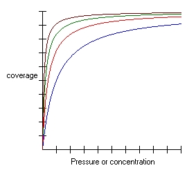
Langmuir equation
Overview

The Langmuir equation or Langmuir isotherm or Langmuir adsorption equation relates the coverage or adsorption of molecules on a solid surface to gas pressure or concentration of a medium above the solid surface at a fixed temperature. The equation was developed by Irving Langmuir in 1916. The equation is stated as:
- <math> \theta =\frac{\alpha \cdot P}{1+\alpha \cdot P}</math>
θ or theta is the percentage coverage of the surface, P is the gas pressure or concentration, α alpha is a constant.
The constant α is the Langmuir adsorption constant and increases with an increase in the strength of adsorption and with a decrease in temperature. The equation is derived starting from the equilibrium between empty surface sites, particles and filled particle sites
- <math> S^* + P \leftrightarrow SP</math>
equilibrium between empty surface sites S* and particles P and filled surface sites SP
- <math> K =\frac{[SP]}{[S^*][P]}</math>
Because the fraction of filled surface sites is equal to θ and the fraction of unfilled sites equal to 1-θ and because P is proportional to the gas pressure or concentration the equation can be rewritten to
- <math> K =\frac{\theta}{(1-\theta)P}</math>
Other equations relating to adsorption exist such as the Temkin equation or the Freundlich equation. The Langmuir equation (as a relationship between the concentration of a compound adsorbing to binding sites and the fractional occupancy of the binding sites) is equivalent to the Hill equation.
Equation Optimization
The Langmuir equation is expressed here as:
- <math> {\Gamma} = \frac{\Gamma_{max} K c}{1 + K c}</math>
where K = Langmuir equilibrium constant, c = aqueous concentration (or gaseous partial pressure), Γ = amount adsorbed, and Γmax = maximum amount adsorbed as c increases. The Langmuir equation can be optimized by linear regression and nonlinear regression methods. Commonly used linear regression methods are: Lineweaver-Burk, Eadie-Hofstee, Scatchard, and Langmuir.
The double reciprocal of the Langmuir equation yields the Lineweaver-Burk equation:
- <math> \frac{1}{\Gamma} = \frac{1}{\Gamma_{max}} + \frac{1}{\Gamma_{max}Kc}</math>
A plot of (1/Γ) versus (1/c) yields a slope = 1/(ΓmaxK) and an intercept = 1/Γmax. The Lineweaver-Burk regression is very sensitive to data error and it is strongly biased toward fitting the data in the low concentration range. It was proposed in 1934. Another common linear form of the Langmuir equation is the Eadie-Hofstee equation:
- <math> \Gamma = \Gamma_{max} - \frac{\Gamma}{Kc}</math>
A plot of (Γ) versus (Γ/c) yields a slope = -1/K and an intercept = Γmax. The Eadie-Hofstee regression has some bias toward fitting the data in the low concentration range. It was proposed in 1942 and 1952. Note that if you invert the x and y axes, then this regression would convert into the Scatchard regression:
- <math> \frac{\Gamma}{c} = K\Gamma_{max} - K\Gamma</math>
A plot of (Γ/c) versus (Γ) yields a slope = -K and an intercept = KΓmax. The Scatchard regression is biased toward fitting the data in the high concentration range. It was proposed in 1949. Note that if you invert the x and y axes, then this regression would convert into the Eadie-Hofstee regression discussed earlier. The last linear regression commonly used is the Langmuir linear regression proposed by Langmuir himself in 1918:
- <math> \frac{c}{\Gamma} = \frac{c}{\Gamma_{max}} + \frac{1}{K\Gamma_{max}}</math>
A plot of (c/Γ) versus (c) yields a slope = 1/Γmax and an intercept = 1/(KΓmax). This regression is often erroneously called the Hanes-Woolf regression. The Hanes-Woolf regression was proposed in 1932 and 1957 for optimizing the Michaelis-Menten equation, which is similar in form to the Langmuir equation. Nevertheless, Langmuir proposed this linear regression technique in 1918, and it should be referred to as the Langmuir linear regression when applied to adsorption isotherms. The Langmuir regression has very little sensitivity to data error. It has some bias toward fitting the data in the middle and high concentration range.
There are two kinds of nonlinear least squares (NLLS) regression techniques that can be used to optimize the Langmuir equation. They differ only on how the goodness-of-fit is defined. In the v-NLLS regression method, the best goodness-of-fit is defined as the curve with the smallest vertical error between the optimized curve and the data. In the n-NLLS regression method, the best goodness-of-fit is defined as the curve with the smallest normal error between the optimized curve and the data. Using the vertical error is the most common form of NLLS regression criteria. Definitions based on the normal error are less common. The normal error is the error of the datum point to the nearest point on the optimized curve. It is called the normal error because the trajectory is normal (that is, perpendicular) to the curve.
It is a common misconception to think that NLLS regression methods are free of bias. However, it is important to note that the v-NLLS regression method is biased toward the data in the low concentration range. This is because the Langmuir equation has a sharp rise at low concentration values, which results in a large vertical error if the regression does not optimize this region of the graph well. Conversely, the n-NLLS regression method does not have any significant bias toward any region of the adsorption isotherm.
Whereas linear regressions are relatively easy to pursue with simple programs, such as excel or hand-held calculators, the nonlinear regressions are much more difficult to solve. The NLLS regressions are best pursued with any of various computer programs.
External links
- Langmuir isotherm @ Queen Mary, University of London Website
- Langmuir isotherm @ http://www.erpt.org Website
- LMMpro, a Langmuir optimization software @ http://www.alfisol.com Website
References
- The constitution and fundamental properties of solids and liquids. part i. solids. Irving Langmuir; J. Am. Chem. Soc. 38, 2221-95 1916 First Page